
Email: chaoran.liu@icloud.com
LinkedIn: sg.linkedin.com/in/liuchaoran
blog in github: https://6chaoran.github.io/data-story
Email: chaoran.liu@icloud.com
LinkedIn: sg.linkedin.com/in/liuchaoran
blog in github: https://6chaoran.github.io/data-story
R users have been complaining about the package version control for a long time. We admire python users, who can use simple commands to save and restore the packages with correct versions.
The good news is that, RStudio recently introduced renv package to manage the local dependency and environment, filling the gap between R and python. renv resembles the conda / virtualenv concept in python.
There are a lot of similarities between renv and python virtual environment.
| task | R with renv | Python with conda | Python with pip |
|---|---|---|---|
| create the environment | renv::init() | conda create | virtualenv |
| save the environment | renv::snapshot() | conda env export > environment.yml | pip freeze > requirements.txt |
| load the environment | renv::restore() | conda env create -f environment.yml | pip install -r requirements.txt |
The latest renv version is 0.11.0 in CRAN, dated by July 19, 2020.
# install from CRAN
install.packages('renv')
The general workflow can be summarized as following:
renv::init()
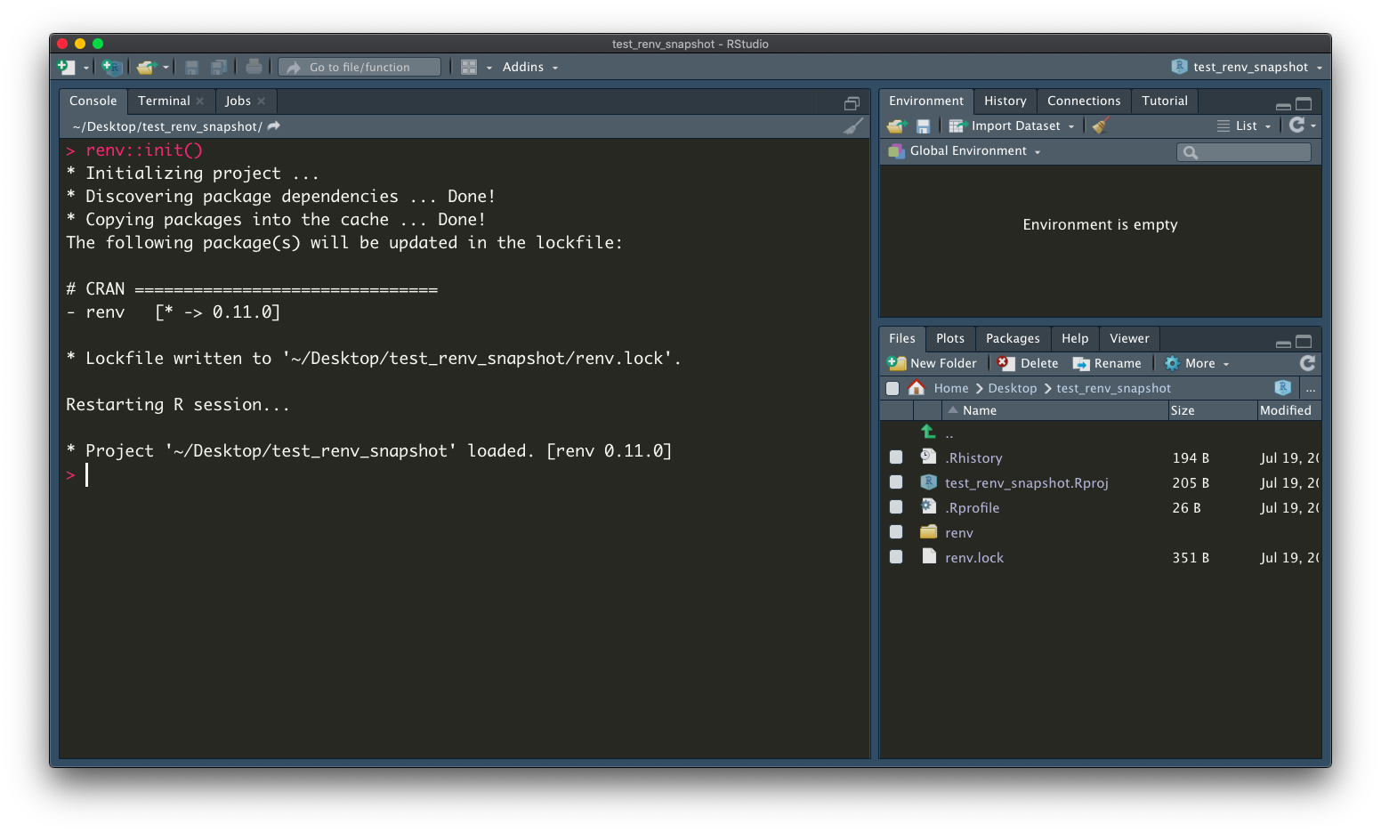
After calling the function, several elements are initialized in the project folder:
renv folder where packages are savedrenv.lock a json file stores the R version, packages detail..Rprofile a source command to activate the environment when the project opensFor example, if we need to install glue and digest package with specific version from CRAN and Github, we can still use install.packages or renv::install function from renv.
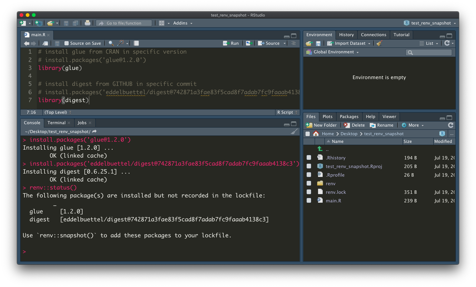
Let’s call renv::status() to check the required packages which are changed, according to the package dependency in your R scripts. Because we library these two packages in our main.R, renv reminds us these two packages not recorded in the renv.lock file.
renv.lock
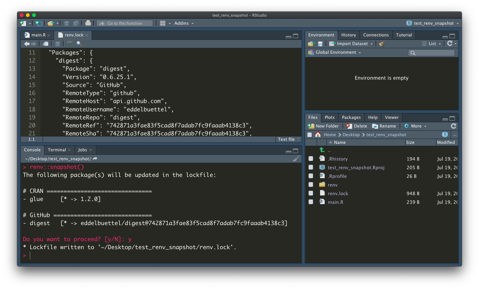
renv::snapshot()
Whenever we want to save the package information into renv.lock, we can call renv::snapshot().
When the code development is done, we can pass the renv.lock file together with the R code to others for collaboration.
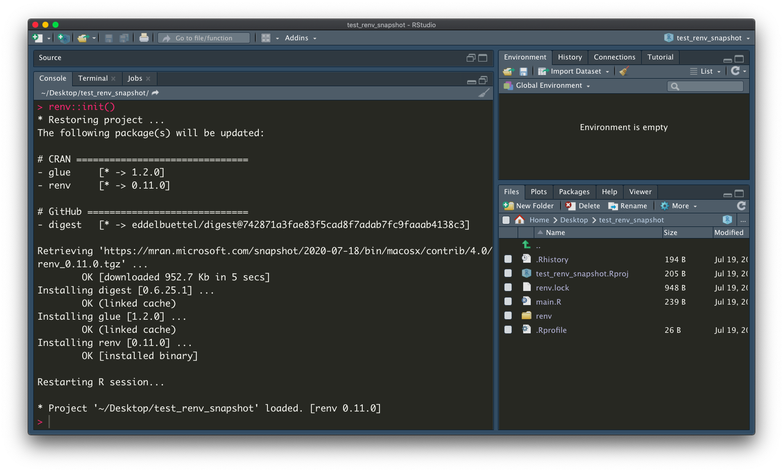
renv.lockWhen the others get the renv.lock file and try to reproduce the development environment, this can be done by following:
# if `renv` is not created yet, using
renv::init()
# if `renv` is already created, using
renv::restore()
Prior the introduction of renv, when we want to containerize R code with docker, we need to create a separate R code which lists all the install.packages commands. Now we can just conveniently call one line of code.
The official document recommends two methods of using renv with docker
pre-baked method: restore packages when docker image built, but can’t use the cached packages and the image building will be slow.cached-mounted method: build the docker image without installing packages, and then mount the cached package library to install the cached packages.I personally still prefer the 1st method, even though it’s slower.
Let’s create a folder call test_renv_restore and copy the renv.lock and main.R from previous folder. Then create a Dockerfile as below:
FROM rocker/r-base:4.0.2
# install renv package
RUN Rscript -e "install.packages('renv')"
# copy everything to docker, including renv.lock file
COPY . /app
# set working directory
WORKDIR /app
# restore all the packages
RUN Rscript -e "renv::restore()"
# run our R code
CMD ["Rscript", "main.R"]
call the docker build using
cd ~/test_renv_restore
docker build -t renv .

renv makes the package management effortless and just one line of code solved the problem.
In this post, we build a model that provides end-to-end capability of detecting faces from image and predicting the BMI, Age and Gender for each detected persons.
The model is made up by several parts:
X)y: {BMI, Age, Gender}) from meta-datagenerator for model fittingMTCNN):
VGGFace):
VGGFace, with VGG16 and ResNet50 backbonesThe architecture of the model is described as below:

Face detection is done by MTCNN, which is able to detect multiple faces within an image and draw the bounding box for each faces.
It serves two purposes for this project:
Prior model training, each image is pre-processed by MTCNN to extract faces and crop images to focus on the facial part. The cropped images are saved and used to train the model in later part.
Illustration of face alignment:

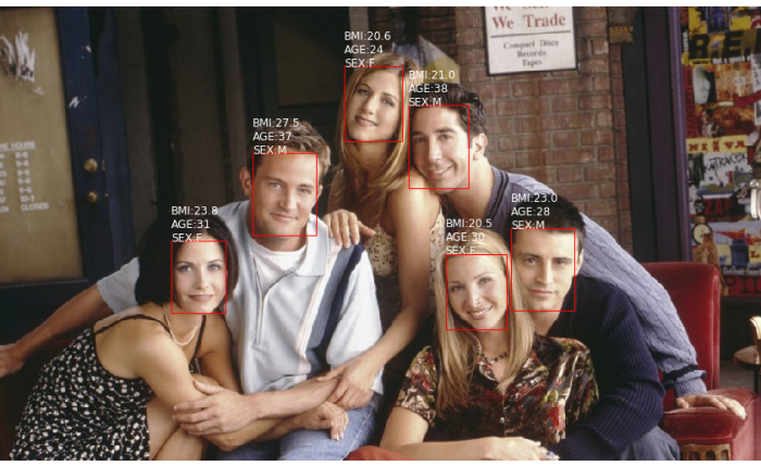
In inference phase, faces will be detected from the input image. For each face, it will go through the same pre-processing and make the predictions.
Illustration of ability to predict for multiple faces:
In vanilla CNN architecture, convolutional blocks are followed by the dense layers to output the prediction. In a naive implementation, we can build 3 models to predict BMI, age and gender individually. However, there is a strong drawback that 3 models are required to be trained and serialized separately, which drastically increases the maintenance efforts.
[input image] => [VGG16] => [dense layers] => [BMI]
[input image] => [VGG16] => [dense layers] => [AGE]
[input image] => [VGG16] => [dense layers] => [SEX]
Since we are going to predict BMI, Age, Sex from the same image, we can share the same backbone for the three different prediction heads and hence only one model will be maintained.
[input image] => [VGG16] => [separate dense layers] x3 => weighted([BMI], [AGE], [SEX])
This is the most simplified multi-task learning structure, which assumed independent tasks and hence separate dense layers were used for each head. Other research such as Deep Relationship Networks, used matrix priors to model the relationship between tasks.
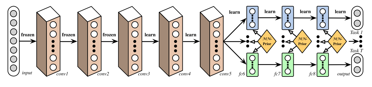 A Deep Relationship Network with shared convolutional and task-specific fully connected layers with matrix priors (Long and Wang, 2015).
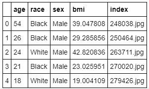
The data used for training was crawled from web. The details of the web-scraping works are recorded in this post: web-scraping-of-javascript-website. This is fairly small dataset, which comprises 1530 records and 16 columns.
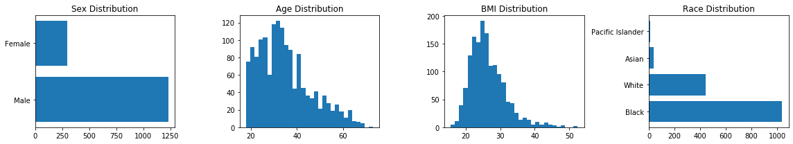
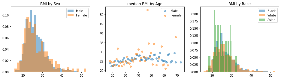
A very brief EDA was done to get the summary of data:
allimages = os.listdir('./face_aligned/')
train = pd.read_csv('./train.csv')
valid = pd.read_csv('./valid.csv')

train = train.loc[train['index'].isin(allimages)]
valid = valid.loc[valid['index'].isin(allimages)]

data = pd.concat([train, valid])
data[['age','race','sex','bmi','index']].head()
fig, axs = plt.subplots(1,4)
fig.set_size_inches((16, 3))
axs[0].barh(data.sex.unique(), data.sex.value_counts())
axs[0].set_title('Sex Distribution')
axs[1].hist(data.age, bins = 30)
axs[1].set_title('Age Distribution')
axs[2].hist(data.bmi, bins = 30)
axs[2].set_title('BMI Distribution')
axs[3].barh(data.race.unique(), data.race.value_counts())
axs[3].set_title('Race Distribution')
plt.tight_layout()
fig, axs = plt.subplots(1,3)
fig.set_size_inches((16, 4))

for i in ['Male','Female']:
    axs[0].hist(data.loc[data.sex == i,'bmi'].values, label = i, alpha = 0.5, density=True, bins = 30)
axs[0].set_title('BMI by Sex')
axs[0].legend()

res = data.groupby(['age','sex'], as_index=False)['bmi'].median()
for i in ['Male','Female']:
    axs[1].scatter(res.loc[res.sex == i,'age'].values, res.loc[res.sex == i,'bmi'].values,label = i, alpha = 0.5)
axs[1].set_title('median BMI by Age')
axs[1].legend()

for i in ['Black','White','Asian']:
    axs[2].hist(data.loc[data.race == i,'bmi'].values, label = i, alpha = 0.5, density=True, bins = 30)
axs[2].set_title('BMI by Race')
axs[2].legend()

plt.show()
A model class FacePrediction was built separately from the notebook. Please refer to here for the details of model.
es = EarlyStopping(patience=3)
ckp = ModelCheckpoint(model_dir, save_best_only=True, save_weights_only=True, verbose=1)
tb = TensorBoard('./tb/%s'%(model_type))
callbacks = [es, ckp, tb]

model = FacePrediction(img_dir = './face_aligned/', model_type = 'vgg16')
model.define_model()
model.model.summary()
if mode == 'train':
    model.train(train, valid, bs = 8, epochs = 20, callbacks = callbacks)
else:
    model.load_weights(model_dir)
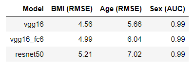
The performance of tested models are quite similar. What surprised me is that, ResNet50 doesn’t outperform VGG16.
Note: VGG16_fc6 is the model that uses VGG16 as backbone, but extracted features from layer fc6 instead of the last convolutional layer. This is recommended setting from this paper: Face-to-BMI: Using Computer Vision to Infer Body Mass Index on Social Media.

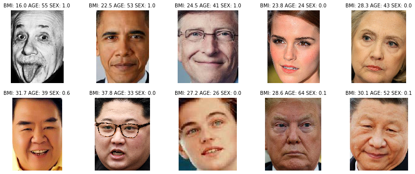
the built model class FacePrediction provides different predict functions
predict from directory:
preds = model.predict('./test_aligned/', show_img = True)
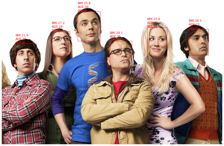
predict multiple faces:
preds = model.predict_faces('./test_mf/the-big-bang-theory-op-netflix.jpg', color = 'red')
predictions from different models: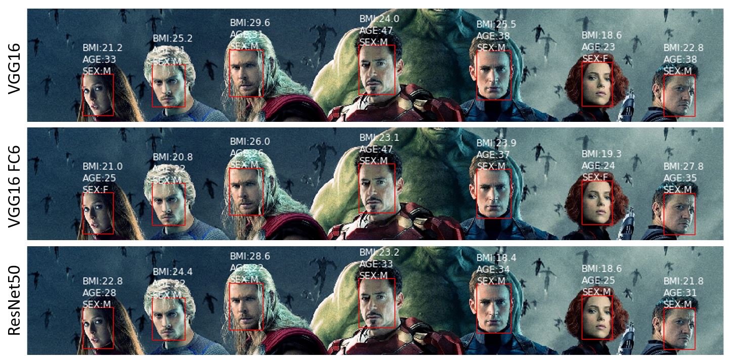
the notebook is available at here
the complete code is available at here
Deep learning / neural network has become a hype and everyone wants to give a try it for better model performance. However, the embarrassed thing is that the neural network sometimes (maybe a lot of times) is not even better than a primitive linear model baseline. I encountered this problem when I tried to do a benchmark of neural network with simple linear model. One of the reasons is that neural network is sensitive to the input distributions and scales, which are not usually addressed when fitting linear models or tree-based models.
Normalization (centred and scaled to unit variance) of input feature space should be able to fix the part of the problem, but it can’t help with deep neural network which could have an effect of “internal co-variate shift” during training. Batch normalization layer is introduced to normalize the output from neural network layers to achieve a faster and stabler convergence.
In this post, I compared a neural network model with linear regression baseline and show how batch normalization layer speeds up the training process.
Continue reading “Stablize your neural network with batch normalization”

In this post, I’m using selenium to demonstrate how to web scrape a JavaScript enabled page.
If you had some experience of using python for web scraping, you probably already heard of beautifulsoup and urllib. By using the following code, we will be able to see the HTML and then use HTML tags to extract the desired elements. However, if the web page embedded with JavaScript, you will notice that some of the HTML elements can’t be seen from the beautiful soup, because they are rendered by the JavaScript. Instead you will only see the script tags, which indicate the place where the JavaScript codes are placed.
Shiny is light-weighted web application, that seamlessly integrated with R. By using shiny, R users can quickly build prototype data product from their existing R models or analysis. In my experience of working with business users, they usually prefer a unified portal, where they can find all analytical solutions provided by data team. Developing a unified shiny application is more preferable, compared with many stand-alone small shiny apps, because the end users don’t have to bookmark the URLs for all applications and are able to access all apps with single login action. It helps to standardize the style and format as well, but on the other hand, it will be more difficult to code and maintain, especially using the default single app.R file structure. Therefore, I’m working on an extendable file structure to build the unified shiny portal.
navbarPage to assemble different shiny apps.paste, useful to format strings.shiny already wraps common HTML tags into shiny tags object. Knowing common HTML tags, such as
div, tags$div()p, tags$p()hr, tags$hr()will be sufficient for this post.
CSS controls the style of HTML elements by Class. This is preferable to create standardized web application, with no harm to your shiny app. CSS formatting file is located under ./www folder for shiny.
In order to make it easy to unit test each individual shiny app, I created directories for each shiny app, where I also have an app.R for testing purpose.
app.R in sub-folder: used for unit testing of this individual shiny app.app.R in main-folder: used for integration testing of unified shiny app.tab.R in sub-folder: used to create a list, that wraps the ui and server of this shiny. After passing the unit test, it can be directly import to main shiny, for integration testing.global.R: used to define global settings, such as database connections, login credentials, page headers/footers.main.css in www-folder: used to define the style of shiny app, by pointing to theme argument in navbarPage. In shiny, the images, css files or JavaScript codes are all located under www folder.
├── 00_tab_login # sub directory for login page
│   ├── app.R # shiny app for unit testing
│   └── tab.R # define a list, wrapping ui and server
├── 01_tab_dashboard_01 # sub directory for dashboard 01
│   ├── app.R
│   └── tab.R
├── 02_tab_dashboard_02 # sub directory for dashboard 02
│   ├── app.R
│   └── tab.R
├── app.R # main shiny app
├── global.R # define global settings
├── readme.md
└── www
    └── main.css # shiny css file

4 directories, 10 files
Using this file structure, I can easily add/remove certain shiny tab, without affecting other components.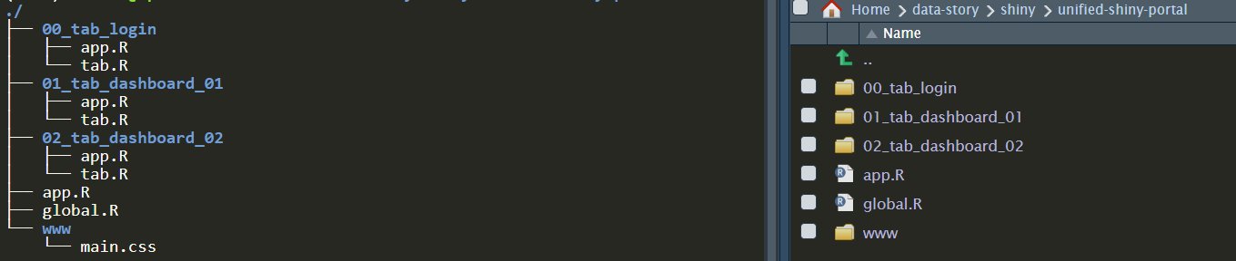
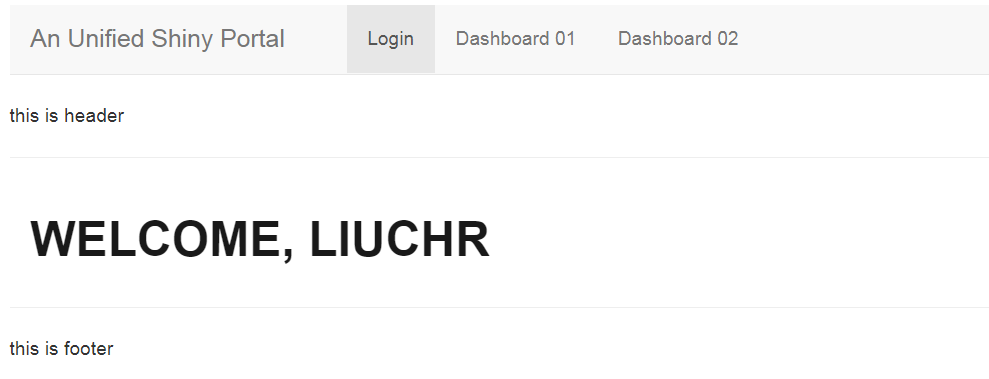
First of all, let’s create a login page to secure our unified shiny app. shiny::modalDialog is used to create the pop-up dialog box, which stops the user accessing the content of shiny app. We just need to add one observeEventon login button to validate the user input. If user input is correct, remove the dialog box and show the welcome message, otherwise keep the dialog box and show the warning message.
The ui component is a tabPanel object, which just contains a hidden welcome message in a div tag.
id is set for shinyjs to locate JavaScript actions on it.class is set for CSS to identify the formatting styles.login_dialog is another ui for the login dialog box, which allows user to input username and password. This UI will be controlled by server.
# define a list to wrap ui/server for login tab
tab_login <- list()

# define ui as tabPanel,
# so that it can be easily added to navbarPage of main shiny program
tab_login$ui <- tabPanel(
  title = 'Login', # name of the tab
  # hide the welcome message at the first place
  shinyjs::hidden(tags$div(
    id = 'tab_login.welcome_div',
    class = 'login-text',
    textOutput('tab_login.welcome_text', container = tags$h2))
  )
)

# define the ui of the login dialog box
# will used later in server part
login_dialog <- modalDialog(
  title = 'Login to continue',
  footer = actionButton('tab_login.login','Login'),
  textInput('tab_login.username','Username'),
  passwordInput('tab_login.password','Password'),
  tags$div(class = 'warn-text',textOutput('tab_login.login_msg'))
)
server component is a function of input,output or session (usually optional), that takes input generated by user and render the changes to output. (Note: user.access is a R list, generated from global.R)
# define the backend of login tab
tab_login$server <- function(input, output) {

  # show login dialog box when initiated
  showModal(login_dialog)

  observeEvent(input$tab_login.login, {
    username <- input$tab_login.username
    password <- input$tab_login.password

    # validate login credentials
    if(username %in% names(user.access)) {
      if(password == user.access[[username]]) {
        # succesfully log in
        removeModal() # remove login dialog
        output$tab_login.welcome_text <- renderText(glue('welcome, {username}'))
        shinyjs::show('tab_login.welcome_div') # show welcome message
      } else {
        # password incorrect, show the warning message
        # warning message disappear in 1 sec
        output$tab_login.login_msg <- renderText('Incorrect Password')
        shinyjs::show('tab_login.login_msg')
        shinyjs::delay(1000, hide('tab_login.login_msg'))
      }
    } else {
      # username not found, show the warning message
      # warning message disappear in 1 sec
      output$tab_login.login_msg <- renderText('Username Not Found')
      shinyjs::show('tab_login.login_msg')
      shinyjs::delay(1000, hide('tab_login.login_msg'))
    }
  })
}
After defined ui and server in tab.R, we now are ready to do the unit testing for shiny login page.
setwd('./00_tab_login')app.R as follow, by assigning the ui and server from tab.R
library(shiny)
library(shinyjs)
library(glue)

source('tab.R') # load tab_login ui/server

ui <- navbarPage(
  title = 'Login',
  selected = 'Login',
  useShinyjs(), # initiate javascript
  tab_login$ui # append defined ui
)

server <- tab_login$server # assign defined server

shinyApp(ui = ui, server = server)
The tested login page
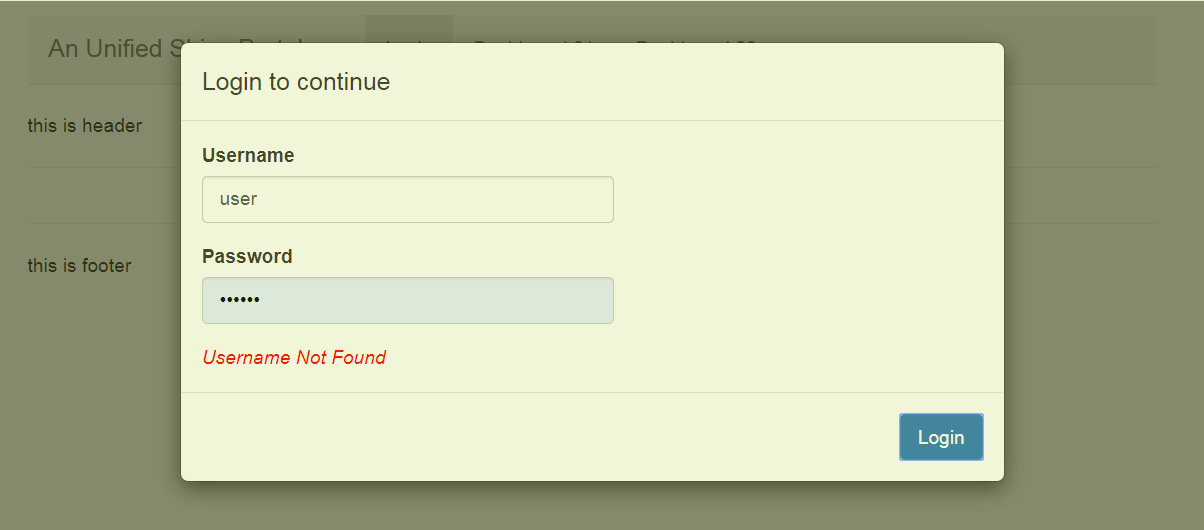
When successfully login, the page should be shown like this:
After login page is tested, I also created two dummy dashboards dashboard 01and dashboard 02.
Similar to 00_tab_login, 01_tab_dashboard_01 and 02_tab_dashboard_02 are structured with tab.R and app.R.
01_tab_dashboard_01: histgram of normal distribution with sample size N (code details)02_tab_dashboard_02: estimation of pi using monte carlo simulation (code details)After component testing of each shiny app is done, we can now put all shiny tabs together to form the unified shiny portal.
library(shiny)
library(shinyjs)
library(glue)

# load global parameters (DB connections, login credentials, etc)
source('global.R')
# load ui/server from each tab
source('./00_tab_login/tab.R')
source('./01_tab_dashboard_01/tab.R')
source('./02_tab_dashboard_02/tab.R')

app.title <- 'A Unified Shiny Portal'

ui <- navbarPage(
  title = app.title,
  id = 'tabs',
  selected = 'Login',
  theme = 'main.css', # defined in www/main.css
  header = header, # defined in global.R
  footer = footer, # defined in global.R
  # initiate javascript
  useShinyjs(),
  # ui for login page
  tab_login$ui,
  # ui for dashboard_01
  tab_01$ui,
  # ui for dashboard_02
  tab_02$ui
)

server <- function(input, output) {

  # load login page server
  tab_login$server(input, output)
  # load server of dashboard_01
  tab_01$server(input, output)
  # load server of dashboard_02
  tab_02$server(input, output)
}

# Run the application
shinyApp(ui = ui, server = server)
the final dashboard 01 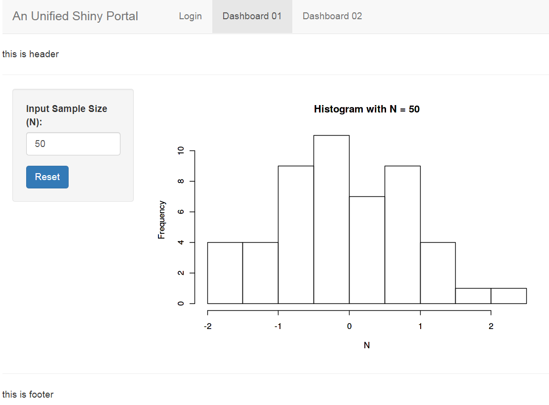
the final dashboard 02 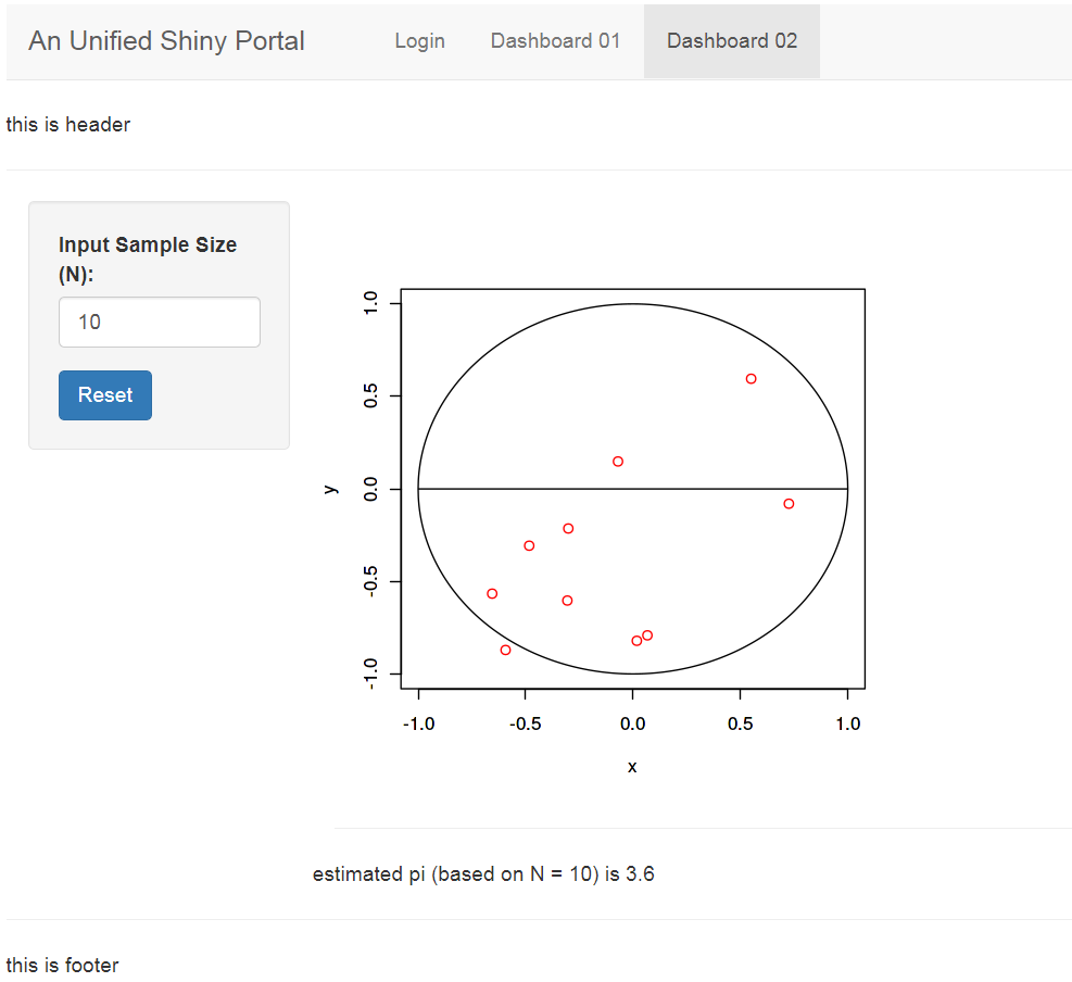
In summary, in order to build a unified shiny portal:
shiny::modalDialog to create dialog box for login pageshiny::showModal,shiny::removeModal,shinyjs to control the dialog box.tab.R defining uiand server and app.R defining code for component testing.ui and server from each tab in app.R of main shiny pagelogin credential ( username: liuchr, password: 123456 )

A set of user-defined functions (UDF) or utility functions are helpful to simplify our code and avoid repeating the same typing for daily analysis work. Previously, I saved all my R functions to a single R file. Whenever I want to use them, I can simply source the R file to import all functions. This is a simple but not perfect approach, especially when I want to check the documentation of certain functions. It was quite annoying that you can’t just type ?func to navigate to the help file. So, this is the main reason for me to write my own util package to wrap all my UDFs with a neat documentation.
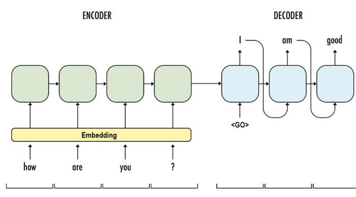
seq2seq model is a general purpose sequence learning and generation model. It uses encoder decoder architecture, which is widely wised in different tasks in NLP, such as Machines Translation, Question Answering, Image Captioning.
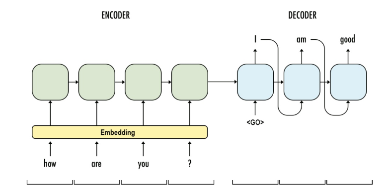
The model consists of major components:
Embedding: using low dimension dense array to represent discrete word token. In practice, a word embedding lookup table is formed with shape (vocab_size, latent_dim) and initialized with random numbers. Then each individual word will look up the index and take the embedding array to represent itself.
Let’s say, if the input sentence is “see you again”, which may be encoded as a sequence of [100, 21, 24]. Each value is the index in the work lookup table. After embedding lookup, the sequence [100, 21, 24] will be converted to [W[100,:], W[21,:], W[24,:]], with W as the word lookup table.
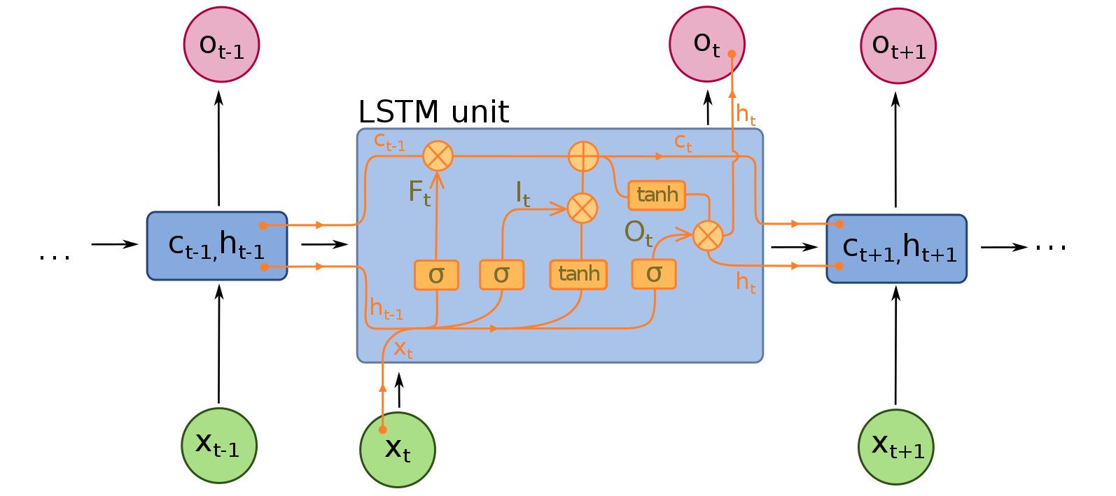
RNN: captures the sequence of data and formed by a series of RNN cells. In neural machine translation, RNN can be either LSTM or GRU.
Encoder: is the a RNN with input as source sentences. The output can be the output array at the final time-step (t) or the hidden states (c, h) or both, depends on the encoder decoder framework setup. The aim of encoder is to capture or understand the meaning of source sentences and pass the knowledge (output, states) to encoder for prediction.
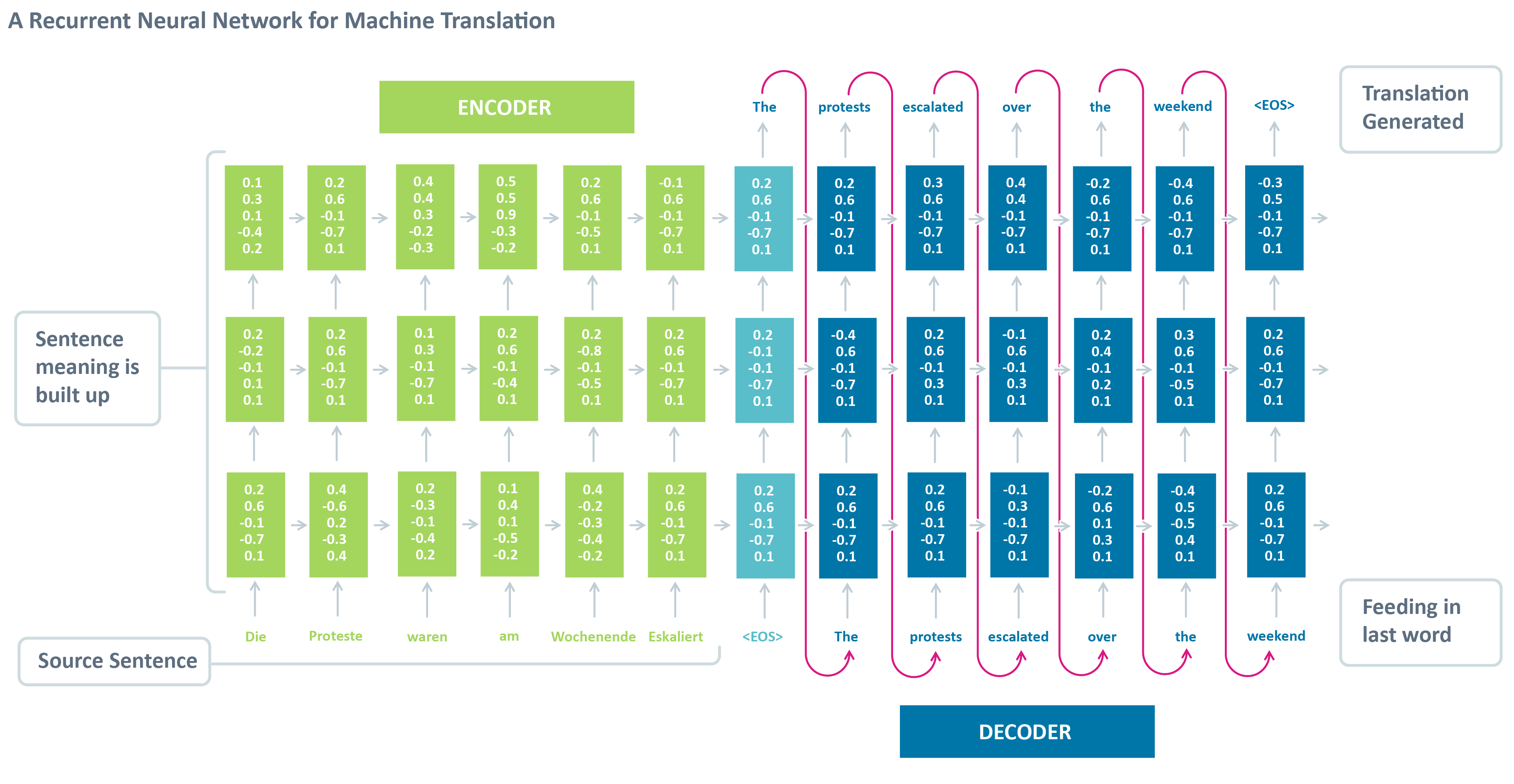
Decoder: is another RNN with input as target sentences. The output is the next token of target sentence. The aim of decoder is to predict the next word, with a word given in the target sentence.
However, we can’t directly use the model for predicting, because we won’t know the decoded sentences when we use the model to translate. Therefore, we need another inference model to performance translation (sequence generation).
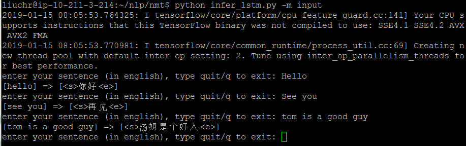
Continue reading “Build a machine translator using Keras (part-1) seq2seq with lstm”
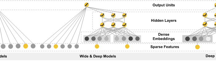
Wide and deep architect has been proven as one of deep learning applications combining memorization and generalization in areas such as search and recommendation. Google released its wide&deep learning in 2016.
Later, on top of wide & deep learning, deepfm was developed combining DNN model and Factorization machines, to further address the interactions among the features.
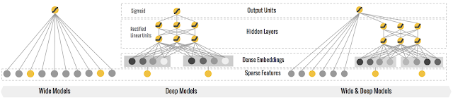

wide&deep learning is logistic regression + deep neural network. In wide part of wide & deep learning, it is a logistic regression, which requires a lot of manual feature engineering efforts to generate the large-scale feature set for wide part.
While the deepfm model instead is factorization machines + deep neural network, as known as neural factorization machines.
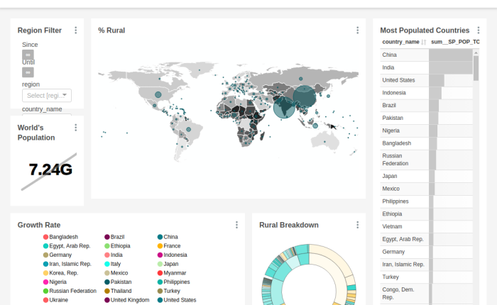

Apache Superset (incubating) is a modern, enterprise-ready business intelligence web application. Compared with business-focused BI tool like Tableau, superset is more technology-navy. It supports more types of visualization and able to work in distributed manner to boost the query performance. Most importantly, it is free of charge!
An example dashboard: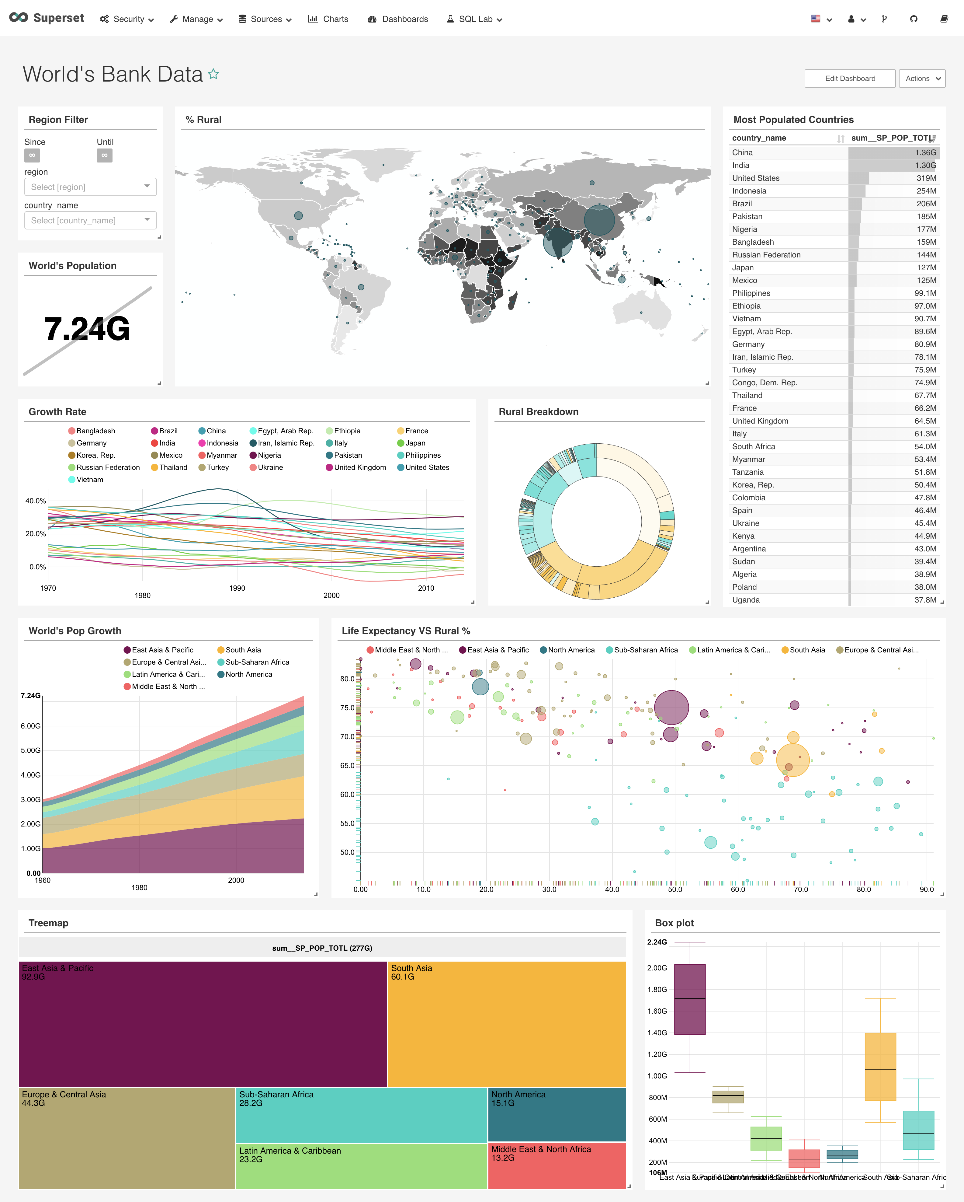
Let’s go and set it up.
The basic tutorial of Keras for R is provided by keras here, which simple and fast to get started. But very soon, I realize this basic tutorial won’t meet my need any more, when I want to train larger dataset. And this is the tutorial I’m going to discuss about keras generators, callbacks and tensorboard.
Continue reading “Not So Basic Keras Tutorial for R – Generators, Callbacks & Tensorboard”
