Detect faces and predict Age, Gender, BMI using Keras

In this post,  we build a model that provides end-to-end capability of detecting faces from image and predicting the BMI, Age and Gender for each detected persons.

The model is made up by several parts:

• input pre-processing pipeline:
  • load the image, resize to 224 x 224 and convert to array, which forms the features (X)
  • map the labels (y: {BMI, Age, Gender}) from meta-data
  • random sample from train and valid dataset to build the generator for model fitting
• face detector (MTCNN):
  • alignment: pre-process the training data by cropping the detected faces
  • detect: when applying the model, detect the bounded faces from input picture and then apply the model for predictions.
• face prediction (VGGFace):
  • transfer learning from VGGFace, with VGG16 and ResNet50 backbones
  • multi-task learning to learn 3 tasks together

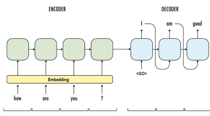
The architecture of the model is described as below:

Face detection

Face detection is done by MTCNN, which is able to detect multiple faces within an image and draw the bounding box for each faces.

It serves two purposes for this project:

1) pre-process and align the facial features of image.

Prior model training, each image is pre-processed by MTCNN to extract faces and crop images to focus on the facial part. The cropped images are saved and used to train the model in later part.

Illustration of face alignment:

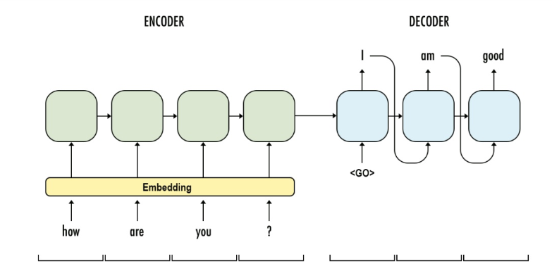
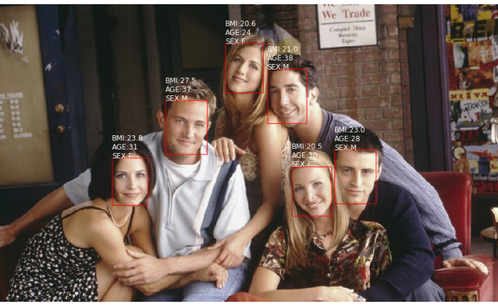
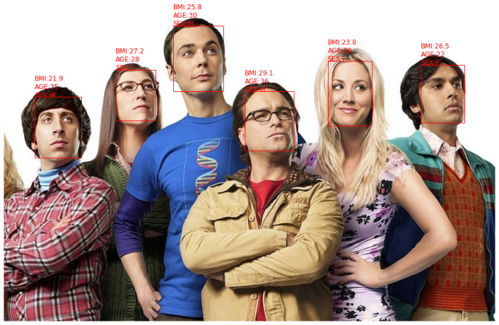
2) enable prediction for multiple persons in the same image.

In inference phase, faces will be detected from the input image. For each face, it will go through the same pre-processing and make the predictions.

Illustration of ability to predict for multiple faces:

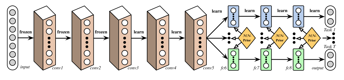
Multi-task prediction

In vanilla CNN architecture, convolutional blocks are followed by the dense layers to output the prediction. In a naive implementation, we can build 3 models to predict BMI, age and gender individually. However, there is a strong drawback that 3 models are required to be trained and serialized separately, which drastically increases the maintenance efforts.

[input image] => [VGG16] => [dense layers] => [BMI]
[input image] => [VGG16] => [dense layers] => [AGE]
[input image] => [VGG16] => [dense layers] => [SEX]

Since we are going to predict BMI, Age, Sex from the same image, we can share the same backbone for the three different prediction heads and hence only one model will be maintained.

[input image] => [VGG16] => [separate dense layers] x3 => weighted([BMI], [AGE], [SEX])

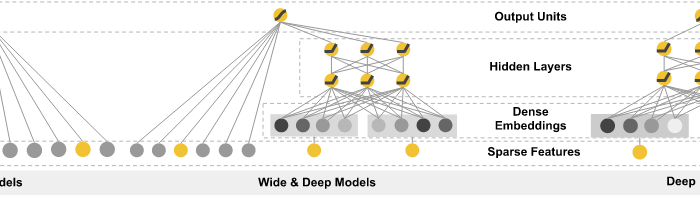
This is the most simplified multi-task learning structure, which assumed independent tasks and hence separate dense layers were used for each head. Other research such as Deep Relationship Networks, used matrix priors to model the relationship between tasks.

A Deep Relationship Network with shared convolutional and task-specific fully connected layers with matrix priors (Long and Wang, 2015).

Dataset

The data used for training was crawled from web. The details of the web-scraping works are recorded in this post: web-scraping-of-javascript-website. This is fairly small dataset, which comprises 1530 records and 16 columns.

A very brief EDA was done to get the summary of data:

• sex imbalance: 80% of the data is male
• age is near truncated normal distribution. min Age is 18, average Age is 34.
• race is dominated by Black and White. Asian samples are very limited.
• BMI is normal distributed, with mean at 26.
• no obvious correlation found between BMI and Age, Sex.

allimages = os.listdir('./face_aligned/')
train = pd.read_csv('./train.csv')
valid = pd.read_csv('./valid.csv')

train = train.loc[train['index'].isin(allimages)]
valid = valid.loc[valid['index'].isin(allimages)]

data = pd.concat([train, valid])
data[['age','race','sex','bmi','index']].head()

fig, axs = plt.subplots(1,4)
fig.set_size_inches((16, 3))
axs[0].barh(data.sex.unique(), data.sex.value_counts())
axs[0].set_title('Sex Distribution')
axs[1].hist(data.age, bins = 30)
axs[1].set_title('Age Distribution')
axs[2].hist(data.bmi, bins = 30)
axs[2].set_title('BMI Distribution')
axs[3].barh(data.race.unique(), data.race.value_counts())
axs[3].set_title('Race Distribution')
plt.tight_layout()

fig, axs = plt.subplots(1,3)
fig.set_size_inches((16, 4))

for i in ['Male','Female']:
    axs[0].hist(data.loc[data.sex == i,'bmi'].values, label = i, alpha = 0.5, density=True, bins = 30)
axs[0].set_title('BMI by Sex')
axs[0].legend()

res = data.groupby(['age','sex'], as_index=False)['bmi'].median()
for i in ['Male','Female']:
    axs[1].scatter(res.loc[res.sex == i,'age'].values, res.loc[res.sex == i,'bmi'].values,label = i, alpha = 0.5)
axs[1].set_title('median BMI by Age')
axs[1].legend()

for i in ['Black','White','Asian']:
    axs[2].hist(data.loc[data.race == i,'bmi'].values, label = i, alpha = 0.5, density=True, bins = 30)
axs[2].set_title('BMI by Race')
axs[2].legend()

plt.show()

Model training

A model class FacePrediction was built separately from the notebook.  Please refer  to here for the details of model.

es = EarlyStopping(patience=3)
ckp = ModelCheckpoint(model_dir, save_best_only=True, save_weights_only=True, verbose=1)
tb = TensorBoard('./tb/%s'%(model_type))
callbacks = [es, ckp, tb]

model = FacePrediction(img_dir = './face_aligned/', model_type = 'vgg16')
model.define_model()
model.model.summary()
if mode == 'train':
    model.train(train, valid, bs = 8, epochs = 20, callbacks = callbacks)
else:
    model.load_weights(model_dir)

Model evaluation

The performance of tested models are quite similar. What surprised me is that, ResNet50 doesn’t outperform VGG16.
Note: VGG16_fc6 is the model that uses VGG16 as backbone, but extracted features from layer fc6 instead of the last convolutional layer. This is recommended setting from this paper: Face-to-BMI: Using Computer Vision to Infer Body Mass Index on Social Media.

Model Predictions

the built model class FacePrediction provides different predict functions

• predict: apply to either single image or a directory, and make subplots
• predict_df: predict from a directory and output as a pandas dataframe
• predict_faces: detect faces and predict for all faces

predict from directory:

preds = model.predict('./test_aligned/', show_img = True)

predict multiple faces:

preds = model.predict_faces('./test_mf/the-big-bang-theory-op-netflix.jpg', color = 'red')

predictions from different models:

Code:

the notebook is available at here
the complete code is available at here

Reference

• MTCNN: https://github.com/ipazc/mtcnn
• VGGFace: https://github.com/rcmalli/keras-vggface
• Face-to-BMI: Using Computer Vision to Infer Body Mass Index on Social Media.

Stablize your neural network with batch normalization

Deep learning / neural network has become a hype and everyone wants to give a try it for better model performance. However, the embarrassed thing is that the neural network sometimes (maybe a lot of times) is not even better than a primitive linear model baseline. I encountered this problem when I tried to do a benchmark of neural network with simple linear model. One of the reasons is that neural network is sensitive to the input distributions and scales, which are not usually addressed when fitting linear models or tree-based models.

Normalization (centred and scaled to unit variance) of input feature space should be able to fix the part of the problem, but it can’t help with deep neural network which could have an effect of “internal co-variate shift” during training. Batch normalization layer is introduced to normalize the output from neural network layers to achieve a faster and stabler convergence.

In this post, I compared a neural network model with linear regression baseline and show how batch normalization layer speeds up the training process.

Build a machine translator using Keras (part-1) seq2seq with lstm

Introduction

seq2seq model is a general purpose sequence learning and generation model. It uses encoder decoder architecture, which is widely wised in different tasks in NLP, such as Machines Translation, Question Answering, Image Captioning.

The model consists of major components:

Embedding: using low dimension dense array to represent discrete word token. In practice, a word embedding lookup table is formed with shape (vocab_size, latent_dim) and initialized with random numbers. Then each individual word will look up the index and take the embedding array to represent itself.

Let’s say, if the input sentence is “see you again”, which may be encoded as a sequence of [100, 21, 24]. Each value is the index in the work lookup table. After embedding lookup,  the sequence [100, 21, 24] will be converted to [W[100,:], W[21,:], W[24,:]], with W as the word lookup table.

RNN: captures the sequence of data and formed by a series of RNN cells. In neural machine translation, RNN can be either LSTM or GRU. 

• t refers to the sequence of the words/tokens.
• x is the input of RNN, refers to the embedding array of the word
• c, h refer to the hidden states from LSTM cells, which is migrating throughout the RNN
• o is the output array, used to map to the predictions

Encoder: is the a RNN with input as source sentences.  The output can be the output array at the final time-step (t) or the hidden states (c, h) or both, depends on the encoder decoder framework setup. The aim of encoder is to capture or understand the meaning of source sentences and pass the knowledge (output, states) to encoder for prediction.

Decoder: is another RNN with input as target sentences.  The output is the next token of target sentence. The aim of decoder is to predict the next word, with a word given in the target sentence.

steps to train a seq2seq model:

1. Word/Sentence representation: this includes tokenize the input and output sentences, matrix representation of sentences, such as TF-IDF, bag-of-words.
2. Word Embedding: lower dimensional representation of words. With a sizeable corpus, embedding layers are highly recommended.
3. Feed Encoder: input source tokens/embedded array into encoder RNN (I used LSTM in this post) and learn the hidden states
4. Connect Encoder & Decoder: pass the hidden states to decoder RNN as the initial states
5. Decoder Teacher Forcing: input the sentence to be translated to decoder RNN, and target is the sentences which is one word right-shifted. In the structure, the objective of each word in the decoder sentence is to predict the next word, with the condition of encoded sentence and prior decoded words. This kind of network training is called teacher forcing.

However, we can’t directly use the model for predicting, because we won’t know the decoded sentences when we use the model to translate. Therefore, we need another inference model to performance translation (sequence generation).

steps to infer a seq2seq model:

1. Encoding: feed the processed source sentences into encoder to generate the hidden states
2. Decoding: the initial token to start is  <s>, with the hidden states pass from encoder, we can predict the next token.
3. Token Search:
   • for each token prediction, we can choose the token with the most probability, this is called greedy search. We just get the best at current moment.
   • alternatively, if we keep the n best candidate tokens, and search for a wider options, this is called beam search, n is the beam size.
   • the stop criteria can be the <e> token or the length of sentence is reached the maximal.

demo of English-Chinese translation

• github repo: https://github.com/6chaoran/nlp/tree/master/nmt
• jupyter notebook: https://github.com/6chaoran/nlp/blob/master/nmt/infer_lstm.ipynb

Implement DeepFM model in Keras

Introduction

Wide and deep architect has been proven as one of deep learning applications combining memorization and generalization in areas such as search and recommendation. Google released its wide&deep learning in 2016.

• wide part: helps to memorize the past behavior for specific choice
• deep part: embed into low dimension, help to discover new user, product combinations

Later, on top of wide & deep learning, deepfm was developed combining DNN model and Factorization machines, to further address the interactions among the features.

wide & deep model

DeepFM model

Comparison

wide&deep learning is logistic regression + deep neural network. In wide part of wide & deep learning, it is a logistic regression, which requires a lot of manual feature engineering efforts to generate the large-scale feature set for wide part.

While the deepfm model instead is factorization machines + deep neural network, as known as neural factorization machines.

Not So Basic Keras Tutorial for R – Generators, Callbacks & Tensorboard

The basic tutorial of Keras for R is provided by keras here, which simple and fast to get started. But very soon, I realize this basic tutorial won’t meet my need any more, when I want to train larger dataset. And this is the tutorial I’m going to discuss about keras generators, callbacks and tensorboard.

Digit Recognition with Tensor Flow

This time I am going to continue with the kaggle 101 level competition – digit recogniser with deep learning tool Tensor Flow.

0. Previously

In the previous post, I used PCA and Pooling methods to reduce the dimensions of the dataset, and train with the linear SVM. Due to the limited efficiency of the R SVM package. I only sampled 500 records and performed a 10-fold cross validation. The resulting accuracy is about 82.7%

1. This Time

With new tool TensorFlow, we can address the problem differently:

• Deep Learning, especially Convolutional Neural Network is well suitable for image recognition problem.
• TensorFlow is a good tool to equickly build the neural network architecture and also empowers the capability of GPUs.
• Convolution Layers artificially create additional features, scanning the boxes of pixel on the image.
• Stochastic Gradient Descent replaces Gradient Descent. SGD takes sample of data to update the gradients, making training fast and less RAM consumption.

Fully utilized the entire dataset (42k records) with deep learning models, the accuracy easily go up above 95%.